Machine Learning in Python#
based on this step by step guide
For today, we will skip most of the theoretical background that goes into machine learning go straight into learning by doing - applying a basic workflow to a dataset to answer some basic questions. If you want to (and you should, if you want to continue using machine learning in the future) learn more about the theoretical backgrounds I reccommend reading Bishop - Pattern Recognition and Machine Learning. Broadly speaking, there are two types of supervised learning models - models for classification and models for regression. What type of model you will use will depend on your specific use case. Today we will focus on classification and apply a basic pipeline to a pre existing dataset

Lets begin by looking at the basic steps of most machine learning projects:
Define Problem.
Prepare Data.
Evaluate Algorithms.
Improve Results.
Present Results.
!pip install -U scikit-learn
Collecting scikit-learn
  Downloading scikit_learn-1.4.0-1-cp311-cp311-macosx_10_9_x86_64.whl.metadata (11 kB)
Requirement already satisfied: numpy<2.0,>=1.19.5 in /Users/aylinkallmayer/anaconda3/envs/pfp_2023-24/lib/python3.11/site-packages (from scikit-learn) (1.26.0)
Requirement already satisfied: scipy>=1.6.0 in /Users/aylinkallmayer/anaconda3/envs/pfp_2023-24/lib/python3.11/site-packages (from scikit-learn) (1.11.3)
Collecting joblib>=1.2.0 (from scikit-learn)
  Using cached joblib-1.3.2-py3-none-any.whl.metadata (5.4 kB)
Collecting threadpoolctl>=2.0.0 (from scikit-learn)
  Using cached threadpoolctl-3.2.0-py3-none-any.whl.metadata (10.0 kB)
Downloading scikit_learn-1.4.0-1-cp311-cp311-macosx_10_9_x86_64.whl (11.5 MB)
   ━━━━━━━━━━━━━━━━━━━━━━━━━━━━━━━━━━━━━━━━ 11.5/11.5 MB 6.6 MB/s eta 0:00:0000:0100:01
?25hUsing cached joblib-1.3.2-py3-none-any.whl (302 kB)
Using cached threadpoolctl-3.2.0-py3-none-any.whl (15 kB)
Installing collected packages: threadpoolctl, joblib, scikit-learn
Successfully installed joblib-1.3.2 scikit-learn-1.4.0 threadpoolctl-3.2.0
import scipy
import numpy as np
import matplotlib as plt
import pandas as pd
import sklearn
We will first load all functions that we will use
# Load libraries
from pandas import read_csv
from pandas.plotting import scatter_matrix
from matplotlib import pyplot as plt
from sklearn.model_selection import train_test_split
from sklearn.model_selection import cross_val_score
from sklearn.model_selection import StratifiedKFold
from sklearn.metrics import classification_report
from sklearn.metrics import confusion_matrix
from sklearn.metrics import accuracy_score
from sklearn.linear_model import LogisticRegression
from sklearn.tree import DecisionTreeClassifier
from sklearn.neighbors import KNeighborsClassifier
from sklearn.discriminant_analysis import LinearDiscriminantAnalysis
from sklearn.naive_bayes import GaussianNB
from sklearn.svm import SVC
Now, lets load the dataset
# Load dataset
url = "https://raw.githubusercontent.com/jbrownlee/Datasets/master/iris.csv"
names = ['sepal-length', 'sepal-width', 'petal-length', 'petal-width', 'class']
dataset = read_csv(url, names=names)
dataset.head()
| sepal-length | sepal-width | petal-length | petal-width | class | |
|---|---|---|---|---|---|
| 0 | 5.1 | 3.5 | 1.4 | 0.2 | Iris-setosa |
| 1 | 4.9 | 3.0 | 1.4 | 0.2 | Iris-setosa |
| 2 | 4.7 | 3.2 | 1.3 | 0.2 | Iris-setosa |
| 3 | 4.6 | 3.1 | 1.5 | 0.2 | Iris-setosa |
| 4 | 5.0 | 3.6 | 1.4 | 0.2 | Iris-setosa |
# descriptions
print(dataset.describe())
       sepal-length  sepal-width  petal-length  petal-width
count    150.000000   150.000000    150.000000   150.000000
mean       5.843333     3.054000      3.758667     1.198667
std        0.828066     0.433594      1.764420     0.763161
min        4.300000     2.000000      1.000000     0.100000
25%        5.100000     2.800000      1.600000     0.300000
50%        5.800000     3.000000      4.350000     1.300000
75%        6.400000     3.300000      5.100000     1.800000
max        7.900000     4.400000      6.900000     2.500000
# class distribution
print(dataset.groupby('class').size())
class
Iris-setosa        50
Iris-versicolor    50
Iris-virginica     50
dtype: int64
Univariate plots#
Remeber, we can also use some basic plotting functions on pandas dataframes! This will give us an even better idea of the data distributions
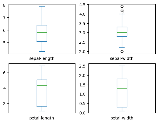
# box and whisker plots
dataset.plot(kind='box', subplots=True, layout=(2,2), sharex=False, sharey=False)
sepal-length       Axes(0.125,0.53;0.352273x0.35)
sepal-width     Axes(0.547727,0.53;0.352273x0.35)
petal-length       Axes(0.125,0.11;0.352273x0.35)
petal-width     Axes(0.547727,0.11;0.352273x0.35)
dtype: object
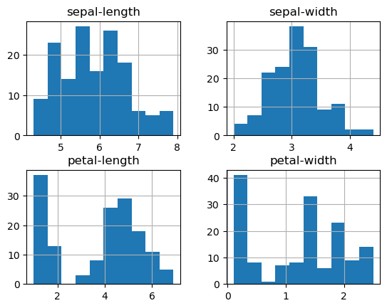
# histograms
dataset.hist()
array([[<Axes: title={'center': 'sepal-length'}>,
        <Axes: title={'center': 'sepal-width'}>],
       [<Axes: title={'center': 'petal-length'}>,
        <Axes: title={'center': 'petal-width'}>]], dtype=object)
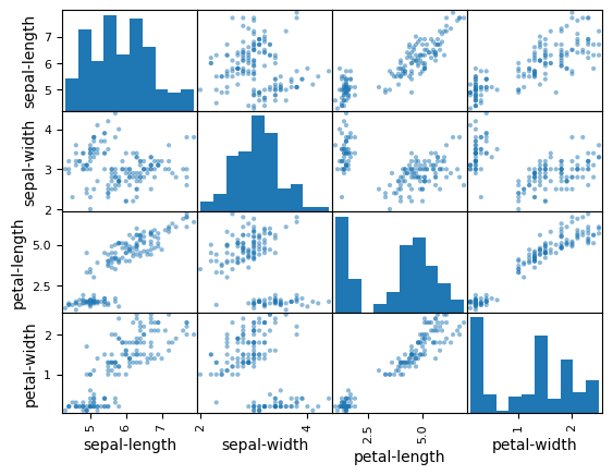
Multivariate plots#
Now we can consider the relationships between different variables
# scatter plot matrix
scatter_matrix(dataset)
array([[<Axes: xlabel='sepal-length', ylabel='sepal-length'>,
        <Axes: xlabel='sepal-width', ylabel='sepal-length'>,
        <Axes: xlabel='petal-length', ylabel='sepal-length'>,
        <Axes: xlabel='petal-width', ylabel='sepal-length'>],
       [<Axes: xlabel='sepal-length', ylabel='sepal-width'>,
        <Axes: xlabel='sepal-width', ylabel='sepal-width'>,
        <Axes: xlabel='petal-length', ylabel='sepal-width'>,
        <Axes: xlabel='petal-width', ylabel='sepal-width'>],
       [<Axes: xlabel='sepal-length', ylabel='petal-length'>,
        <Axes: xlabel='sepal-width', ylabel='petal-length'>,
        <Axes: xlabel='petal-length', ylabel='petal-length'>,
        <Axes: xlabel='petal-width', ylabel='petal-length'>],
       [<Axes: xlabel='sepal-length', ylabel='petal-width'>,
        <Axes: xlabel='sepal-width', ylabel='petal-width'>,
        <Axes: xlabel='petal-length', ylabel='petal-width'>,
        <Axes: xlabel='petal-width', ylabel='petal-width'>]], dtype=object)
Evaluate some algorithms#
Training and validation should always be seperated i.e. should not be performed on the same data. We will therefore split the loaded dataset into two, 80% of which we will use to train, evaluate and select among our models, and 20% that we will hold back as a validation dataset.
# Split into train and validation dataset
array = dataset.values
X = array[:,0:4]
y = array[:,4]
X_train, X_validation, Y_train, Y_validation = train_test_split(X, y, test_size=0.20, random_state=1)
We will use stratified 10-fold cross validation to estimate model accuracy. This will split our dataset into 10 parts, train on 9 and test on 1 and repeat for all combinations of train-test splits. Stratified means that each fold or split of the dataset will aim to have the same distribution of example by class as exist in the whole training dataset.
We are using the metric of ‘accuracy‘ to evaluate models. This is a ratio of the number of correctly predicted instances divided by the total number of instances in the dataset multiplied by 100 to give a percentage (e.g. 95% accurate). We will be using the scoring variable when we run build and evaluate each model next.
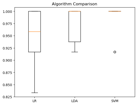
Let’s test 3 different algorithms:
Logistic Regression (LR)
Linear Discriminant Analysis (LDA)
Support Vector Machines (SVM)
# Spot Check Algorithms
models = []
models.append(('LR', LogisticRegression(solver='liblinear', multi_class='ovr')))
models.append(('LDA', LinearDiscriminantAnalysis()))
models.append(('SVM', SVC(gamma='auto')))

models
[('LR', LogisticRegression(multi_class='ovr', solver='liblinear')),
 ('LDA', LinearDiscriminantAnalysis()),
 ('SVM', SVC(gamma='auto'))]
# evaluate each model in turn
results = []
names = []
for name, model in models:
	kfold = StratifiedKFold(n_splits=10, random_state=1, shuffle=True)
	cv_results = cross_val_score(model, X_train, Y_train, cv=kfold, scoring='accuracy')
	results.append(cv_results)
	names.append(name)
	print('%s: %f (%f)' % (name, cv_results.mean(), cv_results.std()))
LR: 0.941667 (0.065085)
LDA: 0.975000 (0.038188)
SVM: 0.983333 (0.033333)
# Compare Algorithms
plt.boxplot(results, labels=names)
plt.title('Algorithm Comparison')
Text(0.5, 1.0, 'Algorithm Comparison')
Make predictions#
We will pick the best performing algorithm - SVM - and test it on the held out validation set. This will give us an independent final check on the accuracy of the best model. It is valuable to keep a validation set just in case you made a slip during training, such as overfitting to the training set or a data leak. Both of these issues will result in an overly optimistic result.
# Make predictions on validation dataset
model = SVC(gamma='auto')
model.fit(X_train, Y_train)
predictions = model.predict(X_validation)
Evaluate predictions#
# Evaluate predictions
print(accuracy_score(Y_validation, predictions))
print(confusion_matrix(Y_validation, predictions))
0.9666666666666667
[[11  0  0]
 [ 0 12  1]
 [ 0  0  6]]
Whats next?#
Want to continue practicing? Keep working on these free, openly available datasets to learn more about the different algorithms, familiarize yourself with data transformations (scaling etc.) and when they are needed.
Interested in reading minds? Want to learn how to decode brains? Start here